
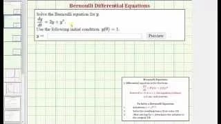
B25 Example problem solving for a Bernoulli equation
See how to solve a Bernoulli equation.
From playlist Differential Equations

Solve a Bernoulli Differential Equation (Part 2)
This video provides an example of how to solve an Bernoulli Differential Equation. The solution is verified graphically. Library: http://mathispower4u.com
From playlist Bernoulli Differential Equations

Illustrates the solution of a Bernoulli first-order differential equation. Free books: http://bookboon.com/en/differential-equations-with-youtube-examples-ebook http://www.math.ust.hk/~machas/differential-equations.pdf
From playlist Differential Equations with YouTube Examples
Ex: Solve a Bernoulli Differential Equation Using an Integrating Factor
This video explains how to solve a Bernoulli differential equation. http://mathispower4u.com
From playlist Bernoulli Differential Equations
Ex: Solve a Bernoulli Differential Equation Using Separation of Variables
This video explains how to solve a Bernoulli differential equation. http://mathispower4u.com
From playlist Bernoulli Differential Equations
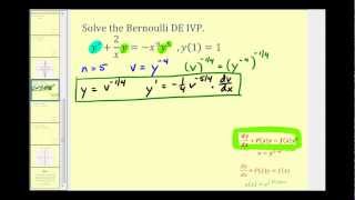
Solve a Bernoulli Differential Equation Initial Value Problem
This video provides an example of how to solve an Bernoulli Differential Equations Initial Value Problem. The solution is verified graphically. Library: http://mathispower4u.com
From playlist Bernoulli Differential Equations
Solve a Bernoulli Differential Equation (Part 1)
This video provides an example of how to solve an Bernoulli Differential Equation. The solution is verified graphically. Library: http://mathispower4u.com
From playlist Bernoulli Differential Equations

Lecture 19: Identification and Falsification
MIT 14.04 Intermediate Microeconomic Theory, Fall 2020 Instructor: Prof. Robert Townsend View the complete course: https://ocw.mit.edu/courses/14-04-intermediate-microeconomic-theory-fall-2020/ YouTube Playlist: https://www.youtube.com/watch?v=XSTSfCs74bg&list=PLUl4u3cNGP63wnrKge9vllow3Y2
From playlist MIT 14.04 Intermediate Microeconomic Theory, Fall 2020

Lecture 3: Income and Substitution Effects
MIT 14.04 Intermediate Microeconomic Theory, Fall 2020 Instructor: Prof. Robert Townsend View the complete course: https://ocw.mit.edu/courses/14-04-intermediate-microeconomic-theory-fall-2020/ YouTube Playlist: https://www.youtube.com/watch?v=XSTSfCs74bg&list=PLUl4u3cNGP63wnrKge9vllow3Y2
From playlist MIT 14.04 Intermediate Microeconomic Theory, Fall 2020

4. Parametric Inference (cont.) and Maximum Likelihood Estimation
MIT 18.650 Statistics for Applications, Fall 2016 View the complete course: http://ocw.mit.edu/18-650F16 Instructor: Philippe Rigollet In this lecture, Prof. Rigollet talked about confidence intervals, total variation distance, and Kullback-Leibler divergence. License: Creative Commons B
From playlist MIT 18.650 Statistics for Applications, Fall 2016

B24 Introduction to the Bernoulli Equation
The Bernoulli equation follows from a linear equation in standard form.
From playlist Differential Equations

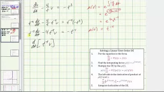
C36 Example problem solving a Cauchy Euler equation
An example problem of a homogeneous, Cauchy-Euler equation, with constant coefficients.
From playlist Differential Equations

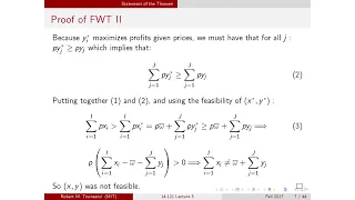
Lecture 20: Failure of Welfare Theorems
MIT 14.04 Intermediate Microeconomic Theory, Fall 2020 Instructor: Prof. Robert Townsend View the complete course: https://ocw.mit.edu/courses/14-04-intermediate-microeconomic-theory-fall-2020/ YouTube Playlist: https://www.youtube.com/watch?v=XSTSfCs74bg&list=PLUl4u3cNGP63wnrKge9vllow3Y2
From playlist MIT 14.04 Intermediate Microeconomic Theory, Fall 2020

Ten Years of "The Wonder of Their Voices": The Future of the Boder Collection
On December 2, 2020, the Fortunoff Video Archive hosted a discussion with author Alan Rosen and Illinois Institute of Technology (IIT) library and archive staff, Adam Strohm and Mindy Pugh, about the work of psychologist and interviewer David Boder. As a faculty member of IIT, Boder interv
From playlist Fortunoff Video Archive for Holocaust Testimonies

MIT 14.04 Intermediate Microeconomic Theory, Fall 2020 Instructor: Prof. Robert Townsend View the complete course: https://ocw.mit.edu/courses/14-04-intermediate-microeconomic-theory-fall-2020/ YouTube Playlist: https://www.youtube.com/watch?v=XSTSfCs74bg&list=PLUl4u3cNGP63wnrKge9vllow3Y2
From playlist MIT 14.04 Intermediate Microeconomic Theory, Fall 2020

9. Parametric Hypothesis Testing (cont.)
MIT 18.650 Statistics for Applications, Fall 2016 View the complete course: http://ocw.mit.edu/18-650F16 Instructor: Philippe Rigollet In this lecture, Prof. Rigollet talked about Wald's test, likelihood ratio test, and testing implicit hypotheses. License: Creative Commons BY-NC-SA More
From playlist MIT 18.650 Statistics for Applications, Fall 2016
Introduction to Theory of Literature (ENGL 300) In this lecture, Professor Paul Fry explores the works of major Russian formalists reviewed in an essay by Boris Eikhenbaum. He begins by distinguishing Russian formalism from hermeneutics. Eikhenbaum's dependency on core ideas of Marxist
From playlist Introduction to Theory of Literature with Paul H. Fry

Jean-Marc Bardet : Asymptotic behavior of the Laplacian quasi-maximum likelihood estimator of...
Abstract : We prove the consistency and asymptotic normality of the Laplacian Quasi-Maximum Likelihood Estimator (QMLE) for a general class of causal time series including ARMA, AR(∞), GARCH, ARCH(∞), ARMA-GARCH, APARCH, ARMA-APARCH,..., processes. We notably exhibit the advantages (moment
From playlist Probability and Statistics
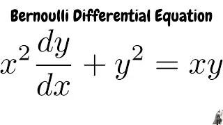
Solving the Bernoulli Differential Equation x^2(dy/dx) + y^2 = xy
Please Subscribe here, thank you!!! https://goo.gl/JQ8Nys How to solve a Bernoulli Differential Equation
From playlist Differential Equations