Autoregressive integrated moving average

Time series models

In statistics and econometrics, and in particular in time series analysis, an autoregressive integrated moving average (ARIMA) model is a generalization of an autoregressive moving average (ARMA) model. Both of these models are fitted to time series data either to better understand the data or to predict future points in the series (forecasting). ARIMA models are applied in some cases where data show evidence of non-stationarity in the sense of mean (but not variance/autocovariance), where an initial differencing step (corresponding to the "integrated" part of the model) can be applied one or more times to eliminate the non-stationarity of the mean function (i.e., the trend). When the seasonality shows in a time series, the seasonal-differencing could be applied to eliminate the seasonal component. Since the ARMA model, according to the Wold's decomposition theorem, is theoretically sufficient to describe a regular (a.k.a. purely nondeterministic) wide-sense stationary time series, we are motivated to make stationary a non-stationary time series, e.g., by using differencing, before we can use the ARMA model. Note that if the time series contains a predictable sub-process (a.k.a. pure sine or complex-valued exponential process), the predictable component is treated as a non-zero-mean but periodic (i.e., seasonal) component in the ARIMA framework so that it is eliminated by the seasonal differencing. The AR part of ARIMA indicates that the evolving variable of interest is regressed on its own lagged (i.e., prior) values. The MA part indicates that the regression error is actually a linear combination of error terms whose values occurred contemporaneously and at various times in the past. The I (for "integrated") indicates that the data values have been replaced with the difference between their values and the previous values (and this differencing process may have been performed more than once). The purpose of each of these features is to make the model fit the data as well as possible. Non-seasonal ARIMA models are generally denoted ARIMA(p,d,q) where parameters p, d, and q are non-negative integers, p is the order (number of time lags) of the autoregressive model, d is the degree of differencing (the number of times the data have had past values subtracted), and q is the order of the moving-average model. Seasonal ARIMA models are usually denoted ARIMA(p,d,q)(P,D,Q)m, where m refers to the number of periods in each season, and the uppercase P,D,Q refer to the autoregressive, differencing, and moving average terms for the seasonal part of the ARIMA model. When two out of the three terms are zeros, the model may be referred to based on the non-zero parameter, dropping "AR", "I" or "MA" from the acronym describing the model. For example, is AR(1), is I(1), and is MA(1). ARIMA models can be estimated following the Box–Jenkins approach. (Wikipedia).

Average velocity vs. average speed

From playlist Sect 3.7, Applications of derivative, (rate of change)

Accelerated motion and oscillation!

In this video i demonstrate accelerated motion with interface. I show the graphs of simple accelerating motion and simple harmonic motion with force and motion sensor!

From playlist MECHANICS

Physics 11.1 Rigid Body Rotation (4 of 10) Calculating Acceleration & Friction of a Car Tire

Visit http://ilectureonline.com for more math and science lectures! In this video I will explain and calculate the acceleration and friction of the tire of a car.

From playlist PHYSICS 11 ROTATIONAL MOTION

QRM 7-2: TS for RM 2 (PACF, ARMA estimation and forecasting)

Welcome to Quantitative Risk Management (QRM). In the second part of Lesson 7, we first introduce the partial autocorrelogram (PACF) and see how we can combine it with the ACF to understand something more about AR, MA and ARMA processes. We then deal with the important problems of estima

From playlist Quantitative Risk Management

Gears and gear ratios: the basics demonstrated and explained: from fizzics.org

The film sets about explaining what gears and gearing can do using practical demonstrations. This includes the working out of gear ratios and speed, the effect of an idler wheel and the use of a two part idler wheel to increase or decrease the speed of the final diven wheel.

From playlist Forces, motion and simple harmonic motion

Time Series Analysis - 2 | Time Series in R | ARIMA Model Forecasting | Data Science | Simplilearn

This Time Series Analysis - 2 in R tutorial will help you understand what is ARIMA model forecasting, what is correlation, and auto-correlation. You will also see a use case implementation in which we forecast sales of air tickets using ARIMA. Finally, we will also look at how to validate

From playlist Data Science For Beginners | Data Science Tutorial🔥[2022 Updated]

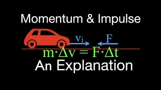
Momentum (5 of 16) Impulse, Example 1

This video goes over an example problem for calculating the change in velocity when an impulse is applied to a moving car. The video also describes the relationship between momentum and impulse. Change in momentum is equal to the impulse. If you apply a force over a period of time then y

From playlist Momentum, Impulse, Inelastic and Elastic Collisions

ARIMA modeling and forecasting | Time Series in Python Part 2

In part 2 of this video series, learn how to build an ARIMA time series model using Python's statsmodels package and predict or forecast N timestamps ahead into the future. Now that we have differenced our data to make it more stationary, we need to determine the Autoregressive (AR) and Mo

From playlist Time Series Forecasting in Python

Time Series class: Part 1 - Dr Ioannis Papastathopoulos, University of Edinburgh

Part 2: https://youtu.be/7n0HTtThMe0 Introduction: Moving average, Autoregressive and ARMA models. Parameter estimation, likelihood based inference and forecasting with time series. Advanced: State-space models (hidden Markov models, Kalman filter) and applications. Recurrent neural netw

From playlist Data science classes

Time Series Talk : ARIMA Model

Intro to the ARIMA model in time series analysis. My Patreon : https://www.patreon.com/user?u=49277905

From playlist Time Series Analysis

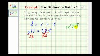
Example 2: Solve a Problem using Distance = Rate x Time

This video provides an example of determining time given the distance and rate. Complete Video List at http://www.mathispower4u.yolasite.com or http://www.mathispower4u.wordpress.com

From playlist Whole Number Applications

Python Live - 1| Time Series Analysis in Python | Data Science with Python Training | Edureka

🔥Python Data Science Training: https://www.edureka.co/data-science-python-certification-course This Edureka Video on Time Series Analysis n Python will give you all the information you need to do Time Series Analysis and Forecasting in Python. Machine Learning Tutorial Playlist: https://g

From playlist Edureka Live Classes 2020

How Manual Transmissions Work! (Animation)

http://www.bring-knowledge-to-the-world.com/ Cars and motorcycles of today are equipped with efficient manual or automatic transmissions. This animation explains manual transmissions. Contents 1) Basic principle of manual transmissions 2) 2-speed manual transmission 3) Gear ratio 4) Shift

From playlist Automotive Engineering

Time Series Analysis | Time Series Forecasting | Time Series Analysis In Excel | Simplilearn

🔥Data Analyst Program (Discount Coupon: YTBE15) : https://www.simplilearn.com/data-analyst-masters-certification-training-course?utm_campaign=TimeSeriesAnalysis-chp71nEc320&utm_medium=Descriptionff&utm_source=youtube 🔥 Professional Certificate Program In Data Analytics: https://www.simplil

From playlist 🔥Data Analytics | Data Analytics Full Course For Beginners | Data Analytics Projects | Updated Data Analytics Playlist 2023 | Simplilearn

Time Series Analysis with the KNIME Analytics Platform

In this session, you’ll learn about the main concepts behind Time Series: preprocessing, alignment, missing value imputation, forecasting, and evaluation. Together we will build a demand prediction application: first with (S)ARIMA models and then with machine learning models. The codeless

From playlist Advanced Machine Learning

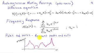
LTI System Models for Random Signals

http://AllSignalProcessing.com for more great signal processing content, including concept/screenshot files, quizzes, MATLAB and data files. Overviews the autoregressive, moving-average, and autoregressive moving-average models for random signals. These describe a random signal as the ou

From playlist Random Signal Characterization

Direct Proportion/Multiplicative Scaling

"Appreciate multiplicative scaling in a variety of contexts, including ingredients."

From playlist Number: Ratio & Proportion

2-3-2 Auto Transitions

R2-D2 2-3-2 transition with automatic center leg control

From playlist Building my life-size R2D2

QRM 7-1: TS for RM 2 (seasons, ARMA and more)

Welcome to Quantitative Risk Management (QRM). Lesson 7 is very rich. In part 1, we start from seasonality and how to deal with it (more applied details in QRM 7-3). We then introduce AR, MA and ARMA processes, discussing their basic properties, like causality and invertibility. To suppo

From playlist Quantitative Risk Management

Calculating Average Drag Force on an Accelerating Car using an Integral

A vehicle uniformly accelerates from rest to 3.0 x 10^1 km/hr in 9.25 seconds and 42 meters. Determine the average drag force acting on the vehicle. Want lecture notes? http://www.flippingphysics.com/drag-force.html This is an AP Physics C Topic. 0:00 Intro 0:14 The Drag Force equation 0:

From playlist Work, Energy, Power, Spring Force - AP Physics C: Mechanics

Autoregressive integrated moving average

Related pages